Ecommerce Shipping Guide

Why Did Your Shipping Costs Rise More Than the Carrier Rate Increase?

The carriers' announced 2026 rate increases looked manageable: roughly 5.9% on average for UPS and FedEx, and about 5 to 8 percent across USPS parcel services [^1][^2]. Budgets were re-forecast, contracts were reviewed, and everyone moved on. Then the invoices came in. Your average quoted cost per parcel did not go up 5.9%. It went up 8%, 12%, sometimes 15% or more, and nobody in the building can say exactly why.

Here is the running example we will use for the rest of this article. Last year your average quoted cost per parcel was $8.20. This year it is $9.65. That is a $1.45 increase, or 17.7%, about three times the announced rate increase. Finance says the carrier repriced us. Operations says it is all surcharges. The warehouse says the parcels did not change. Customer service sees the reships and refunds and quietly wonders how much of that number is rework. None of them is wrong, and none of them can prove it, because each one is holding a different slice of the same cost chain.

The question that actually matters is not “how much did shipping go up” but “why did it go up more than the announced number.” Answering that requires period-over-period attribution, not another horizontal list of causes. And before you attribute anything, you have to separate three observation lenses that most teams collapse into one: the quoted label cost, the final invoiced cost, and the cost per successful delivery. Quote can be cheaper than invoice, and invoice can look fine while failed deliveries quietly destroy the real number.

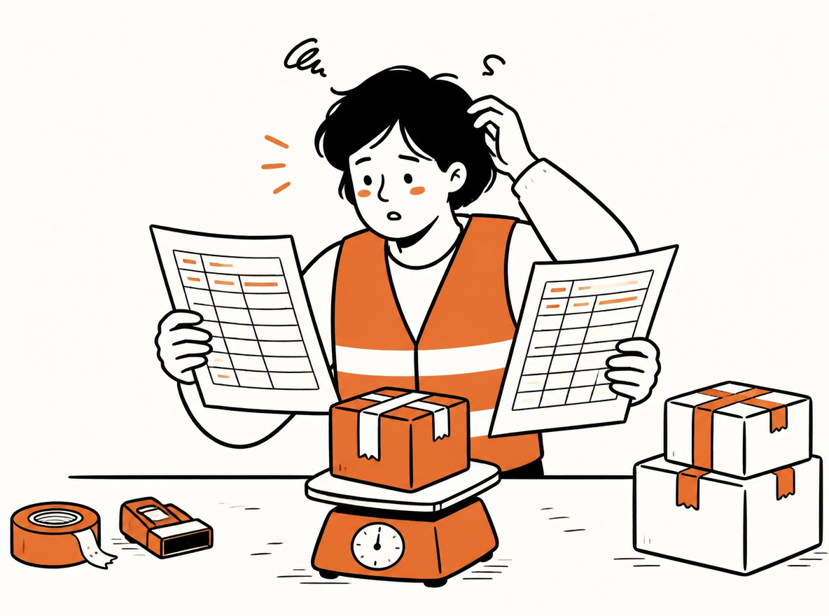
Logistics and finance managers examine a large rising invoice beside a rate card and parcel.
Your bill rose more than the rate card. Everyone sees the number; nobody sees the whole cost chain

The Puzzle: Your Bill Rose More Than the Rate Card Did

Start by seeing the problem clearly. UPS and FedEx announced roughly 5.9% average increases for 2026, and USPS about 5 to 8 percent across parcel services [^1][^2]. That is a rate-card number. But you do not pay the bill line by line against the rate card; you pay it as an average cost per parcel, and that average is pushed by three families of variables at once: Price (rate card, fuel, surcharge rules, account terms), Mix (the share of weight, DIM, SKU, zone, carrier, and service), and Execution (packaging deviations, address corrections, manual overrides, billing adjustments). The announced number only describes part of the first family. That is where the gap comes from.

The traditional way to handle “shipping went up” is to check the rate card: whatever was announced, redo the budget by that number. That works in a single-variable world, but your bill lives in a multi-variable one. Instead of guessing, figure out the magnitude of each effect first, then decide who to talk to and what to change. This is also the difference between this framework and a causes-list article like why your shipping cost is so high: the list tells you what fees exist, attribution tells you where every extra dollar of this specific increase went.

Why Comparing Two Averages Tells You Nothing

The most tempting analysis is also the most useless one: compare last year's average cost per parcel to this year's and call the difference “the rate increase.” An average cost per parcel is a weighted mixture, not a price. It moves when the price list moves, and it moves just as hard when the mix of what you ship moves, and it moves again when the way you execute changes. One number, three families of causes.

Price. The rate card, fuel, the surcharge schedule, and the terms on your account. This is what the carrier announced and what your contract actually says.

Mix. The share of parcels by weight, DIM, SKU, zone, carrier, and service. If this year's orders are heavier, more dimensional-weight-heavy, or shipping to farther zones than last year's, your average rises even with an identical rate card.

Execution. Packaging deviations, address corrections, wrong service selections, manual overrides, and billing adjustments. These are costs your own operation creates after the rate decision, and they show up on the invoice as line items nobody planned for.

Compare two averages and you get one blended number that cannot answer the only question anyone cares about: who owns this increase. The same $1.45 move could be pure price, pure mix, pure execution, or any combination, and the average will look identical in every case. You have to decompose it. If your quote and your final charge keep disagreeing, start with why your shipping quote does not match the final charge; if the reconciliation chain itself is the problem, follow the shipping reconciliation process.

The Parcel Cost Variance Bridge

The Parcel Cost Variance Bridge breaks the gap between two periods into a chain of additive effects, each one an independent explanation of part of the total:

Previous-period cost → Price effect → Parcel-mix effect → Zone effect → Service effect → Carrier-routing effect → Execution effect → Current-period cost. Strip the effects in order and they sum exactly to the total gap.

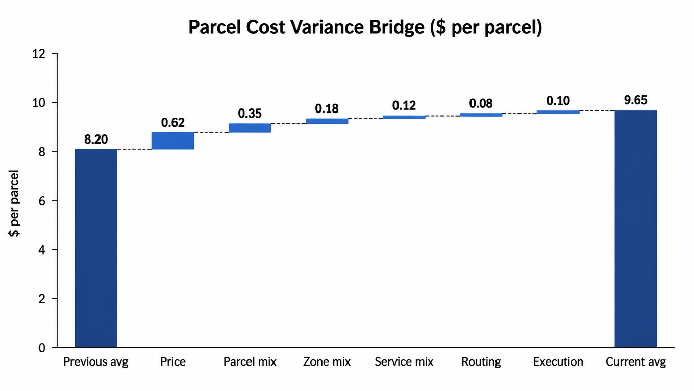
Applied to our example, the $1.45 bridge breaks down as follows. The price effect, from the new rate card, fuel, and surcharge schedule on the same parcels, contributes $0.62. The parcel-mix effect, from heavier and more DIM-heavy orders, contributes $0.35. The zone effect adds $0.18 as more orders travel to farther zones. The service effect adds $0.12 from a shift toward more expedited and guaranteed services. The carrier-routing effect adds $0.08 from routing rules steering more parcels toward a more expensive carrier on the same lanes. The execution effect contributes $0.10 in address corrections, manual overrides, and billing adjustments. $0.62 + $0.35 + $0.18 + $0.12 + $0.08 + $0.10 = $1.45, which closes the bridge exactly.

Waterfall chart: previous average $8.20, plus price $0.62, parcel mix $0.35, zone $0.18, service $0.12, routing $0.08, execution $0.10, equals current average $9.65, a $1.45 gap that closes exactly
The bridge: six effects sum exactly to the total gap

Report the bridge in both dollars per parcel and as a percentage of the prior-period cost, because finance and operations read the same story differently. Finance wants the dollars and the direction; operations wants to know which line they control. In our example, price is 43% of the total variance, mix effects together are 45%, and execution is 7%. A team that negotiates rates to fix the whole $1.45 would be negotiating against a problem that is barely half price.

Build a Matched Cohort Before You Compare Anything

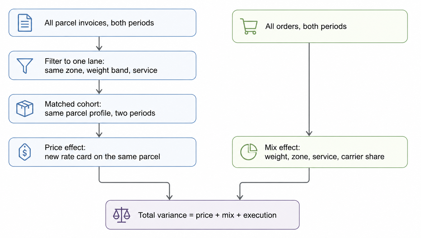
The first step is never the grand average. The first step is to build a matched cohort: take the same lane (same origin, same zone), the same weight band, and the same service, and compare those parcels across the two periods. Only inside a matched cohort does the difference between two averages actually represent price. Everything outside it is structure.

A workable cohort needs at minimum these fields, pulled from the carrier invoice and your WMS or shipping system: carrier and service; origin and destination ZIP or zone; actual weight; package dimensions and DIM weight; SKU or package profile; residential or commercial destination; base charge; fuel and accessorial codes; promised delivery speed; final carrier adjustment; delivery outcome; and the return, reship, or claim outcome.

Then run two steps and present them separately. First, measure the price change inside the matched cohort: same parcel, new rate card. Second, measure the structural change across all orders: how weight, DIM, zone, service, and carrier share moved between periods. If you blend these two steps into one number, you are back to comparing averages and learning nothing.

Flowchart: all parcel invoices for both periods → filter to one lane (same zone, weight band, service) → matched cohort → price effect; and all orders → mix effect; both feed total variance = price + mix + execution
Price is measured inside the cohort, mix across all orders, presented separately

Three traps manufacture fake increases. Peak-season volume mixed into an off-peak comparison inflates the average with a service and weight mix you never see in normal months. New SKUs mixed into the old population add heavier or more DIM-heavy parcels and look like price. And comparing across zones, or across carriers with different zone structures, turns geography into an apparent rate increase. The matched cohort exists to keep these out.

Build comparable periods and action records across clients and facilities

Use the existing variance bridge to explain the change, and include client and facility when applying it to a 3PL. Separate total-spend movement from unit-cost movement: more volume can increase spend without increasing cost per order. New clients, more distant zones, or faster promises are not automatically carrier price increases.

Comparison controlRecommended recordWhen evidence is incomplete
Consistent amount and periodState whether quotes or final charges are compared; align billing periods, currency, tax, and adjustment allocation.List excluded invoices and withhold a realized-savings conclusion.
Matched client and parcel segmentBuild comparable groups by client, facility, service, destination, and measured parcel profile.Report new or disappearing segments separately rather than forcing a match.
A reconciled variance bridgeReconcile component effects to the total and state decomposition order and interaction allocation.Retain unexplained residuals instead of automatically assigning them to pricing or execution.
Action ownershipAssign owners and retest segments separately for packaging, service rules, billing disputes, and contract terms.Gather evidence before changing several variables at once.

Price movement needs an effective quote or contract; invoice movement needs actual charge evidence. Investigate shipment gaps with quote vs. final charge, close invoices and credits through shipping reconciliation, and verify the result with cost per successful delivery while monitoring the client promise.

For a specific weight or dimension error identified by the bridge, reconcile first and use the weight adjustment dispute workflow. Keep differences with incomplete records pending.

What Each Variance Driver Means for Your Next Move

Attribution without action is a post-mortem. Once the bridge tells you where the variance lives, the decision table tells you what to do about it, and whether carrier comparison or routing can actually solve it.

Primary variance source What it means Move Solved by carrier comparison / routing?
Base rate / contract changeThe rate card or contract repriced the same parcelRenegotiate, or compare platform rates against your own accountComparison yes; renegotiation is a contract step
Surcharge schedule changeFuel, DIM, residential, or delivery-area surcharges shiftedCompare all-in cost, never the headline discountYes
DIM / package mixParcels got heavier or more DIM-heavy, or packaging driftedFix packaging, SKU package profiles, warehouse box rulesNo: ops fix; comparison only validates
Zone mixMore orders shipping to farther zonesAdjust warehouse distribution, or test regional carriers on those zonesYes: routing
Service mixMore expedited or guaranteed servicesRecheck the checkout promise against the actual carrier service mappingNo: checkout and operations
Carrier-routing mixRouting rules shifted share toward a more expensive carrierMulti-carrier rate comparison on representative ordersYes: routing
Execution / dataAddress corrections, manual overrides, billing adjustmentsAudit WMS parcel data, address quality, and the override workflowNo: data and process
Delivery failuresFailed attempts, reships, claims inflate true costSwitch to cost per successful delivery, not label pricePartially

The right-hand column is the discipline. If the variance is a packaging problem, negotiating a better discount fixes nothing. If it is a zone problem, the cheapest carrier on your overall average may be the most expensive one on your fastest-growing lane. Match the driver to the tool: contract-level issues deserve a full parcel carrier contract audit, routing-level issues belong inside a multi-carrier shipping strategy, and failed deliveries should be measured with cost per successful delivery.

The Variance Worksheet You Can Copy

The worksheet below is designed to be copied into a spreadsheet and filled from three sources: carrier invoices for both periods, WMS or shipping-system data for both periods, and a manual sample for execution items like packaging and address corrections.

Two formulas do the work. The price effect holds volume at the current period and isolates the rate-card change: (current rate − prior rate) × current volume. The mix effect holds rates at the prior period and isolates the structure change, repeated once per dimension: (current volume − prior volume) × prior rate, applied per weight band, per zone, per service, and per carrier. Because the price effect uses current volume and the mix effects use prior rates, the effects add up exactly to the total variance with no leftover interaction term, which means your worksheet always balances.

Step What to pull Source Example
1. Prior-period costTotal final invoiced parcel cost, all lanesCarrier invoice / billing file$8.20 per parcel average
2. Current-period costSame definition, current periodCarrier invoice / billing file$9.65 per parcel average
3. Price effect(Current rate − prior rate) × current volume, per matched laneRate cards both periods + WMS volume+$0.62
4. Parcel-mix effect(Current volume − prior volume) × prior rate, per weight / DIM bandWMS parcel data+$0.35
5. Zone effectMix formula repeated per zoneWMS + invoice zone fields+$0.18
6. Service effectMix formula repeated per serviceWMS+$0.12
7. Routing effectMix formula repeated per carrierInvoice+$0.08
8. Execution effectManual sample: address corrections, overrides, adjustmentsFinance / billing review+$0.10
9. CheckSum of effects equals total varianceFormula$1.45 = $1.45 ✓

Keep one lane per row in the real worksheet and roll the lanes up only at the end. The minute you average lanes together you are back to the blended number that started this problem.

Diagnosis Is Only Half: Validate the Fix on Your Own Parcel Profile

The variance bridge tells you where the money went, but it does not tell you which fix is actually cheaper. A rate-card comparison on your average parcel can confirm the price effect and mislead you on everything else, because the price effect is only part of the story. The fix has to be validated the same way the diagnosis was built: on your own parcel profile, lane by lane.

Warehouse operator compares two quotations beside a parcel on a scale.
Compare carriers on the same real parcel profile

Work from the cohorts the bridge already gave you. Pick representative ZIP, weight, DIM, and service cohorts from the variance analysis, and compare USPS against the applicable regional carrier options on the exact same shipment profile. Run a small set of real orders through the portal before you change any routing logic, and treat the routing rules as provisional until the final invoiced cost and delivery outcome confirm the comparison. Only when the routing logic is stable and manual decisions become the bottleneck should you consider API automation. And always conclude on the final invoiced cost and delivery outcome, never on the homepage discount number, because discount is a price-effect number and your problem was never only price.

When you are ready to act, use our shipping rate calculator to put candidate carrier rates on one table for the same parcel profile, run the shipping cost optimization advisor to check whether shipping is eating too much of GMV, and see our pricing page for how a channel-neutral shipping layer like EasyShippingX (which compares US domestic carrier options uniformly and executes through a portal, Excel, or API) fits this validation step as the data foundation: run real orders on your cohorts through the portal first, and only consider the API once routing is stable.

The reason your bill outpaced the rate card is that price, structure, and execution all moved at once, and each of those moves has an owner. Attribution locates the problem; comparison validates the fix. That validation belongs on your real parcels, on your real lanes, against the carriers that actually serve them. That is the point where a carrier comparison on your own profile stops being an exercise and becomes the number you take into the next budget cycle.

FAQ

Because the announced number only describes part of the price effect, while your bill moves with price, mix, and execution at the same time. In our example, price is only 43% of the total variance, mix effects together are 45%, and execution is 7%. Decompose the gap with the bridge and a matched cohort, and you can see where every dollar went instead of guessing at a blended average.
Quoted label cost is the price you see in the system, final invoiced cost is what the bill actually charges, and cost per successful delivery folds in failed attempts, reships, and claims. Quote can be cheaper than invoice, and invoice can look fine while failed deliveries quietly raise the real number. Keep the three lenses separate, or you will blur “quotes got more expensive,” “charges got more expensive,” and “failed deliveries made the total more expensive” into one problem.
Start with a matched cohort: same lane, same weight band, same service, across the two periods. Price effect = (current rate − prior rate) × current volume; mix effect = (current volume − prior volume) × prior rate, repeated per weight band, zone, service, and carrier. Because the price effect uses current volume and the mix effects use prior rates, the two add up exactly to the total variance and the worksheet always balances.
Because an average cost per parcel is a weighted mixture, not a price. The same difference could be pure price, pure mix, pure execution, or any combination, and the average looks identical in every case. Worse, mixing in peak-season volume, new SKUs, or different zones manufactures increases that never happened. Build a matched cohort and decompose the bridge first, and you will know who actually owns this increase.
Match the driver to the tool: base rate or contract changes go to renegotiation or platform-rate comparison; surcharge changes to all-in-cost comparison; DIM mix to packaging; zone mix to warehouse distribution or regional carriers; routing mix to multi-carrier comparison; execution and data to a WMS and address-quality audit; failed deliveries to cost per successful delivery. Then validate the fix on your own real parcel profile, cohort by cohort, concluding on final invoiced cost and delivery outcome rather than the homepage discount.
What if the variance bridge cannot explain the full period change?

Retain the unexplained residual, identify missing records/rates/decomposition rules, and assign evidence collection. Do not automatically classify it as carrier repricing or execution error.