Returns Routing Guide

Which Warehouse Should Receive a Return? Compare Shipping Cost, Restock Time, and Recovery Value

Outbound routing is a promise problem. You pick the warehouse that hits the delivery date at the lowest cost, and you can plan it weeks ahead. Reverse routing is a triage problem. The parcel shows up unannounced, in unknown condition, and the right answer depends on what is inside the box, not just where it came from.

The common failure is to open the rate table, find the cheapest return leg, and route there. Return shipping is only one of four lines that decide this, and on a surprising number of SKUs it is not the line that decides anything. The other three are the processing fee, the transfer cost of moving goods a second time, and the value you actually recover once the unit is sellable again.

For a 3PL running several warehouses for merchant clients, this matters twice over. You have to make the routing call, and you have to explain the charge. This is a working method for both, built on one rule: first remove the nodes that cannot handle the goods, then do the arithmetic.

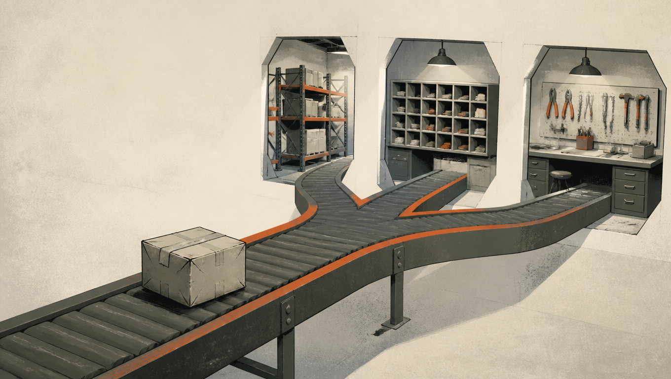
Editorial illustration of a returns conveyor splitting into three lanes that lead into three warehouse interiors in cutaway view, a battered carton riding the belt in the foreground, hand-inked linework, restrained palette with a single orange accent, deliberately off-center composition.
One inbound stream, three exits, three node roles

Gate zero: screen out the nodes that cannot receive or process this SKU

Every comparison starts with subtraction. A node that cannot legally, physically, or procedurally take this SKU does not belong in the scorecard and does not belong in a quote. Putting it there to look competitive is the fastest way to lose a merchant account, because the failure surfaces weeks later as a destroyed unit, an unshippable pallet, or a compliance letter.

Four gates, in order. The first is whether the SKU is returnable at all. Lithium batteries and standalone power banks, aerosols, liquids, hazmat, temperature-controlled goods, activated electronics with a registered serial number, and anything with a manufacturer policy against resale of opened units all carry restrictions that vary by carrier and by node. FedEx, for one, will not accept recalled or defective batteries or waste batteries moving for recycling or disposal (FedEx battery shipping rules), and USPS publishes its own mailability rules for aerosols, liquids, and other hazardous materials (USPS Publication 52). The second gate is whether the buyer's return channel can actually reach a candidate node: is the ZIP in the pickup area, can the carrier hand a label to the buyer, does the return lane share a line with your outbound freight. The third gate is whether that specific node can receive and process the category properly: an evidence bench for damage claims, a functional test rig, refurbishment capability, hazmat storage, a permit for e-waste disposal, or the approved space to hold units pending destruction. E-waste handling is regulated rather than optional: the EPA treats cathode ray tubes and their glass as hazardous waste when disposed, and only excludes them from that definition if they are genuinely being reused or recycled (EPA guidance on cathode ray tubes).

Only after a node clears those three does the fourth gate open, and that is total economics. The ordering is not a formality. A cheap node that cannot process a battery pack is not a cheap option, it is an unavailable one, and no quoted rate changes that. Write the gate result into the same row as the cost lines, including the exclusion reason, so the decision survives an audit six months later.
Three node roles: direct-to-fulfillment, centralized hub, specialized processing

The nodes you are choosing between are not interchangeable warehouses of different sizes. They are three roles, and they differ in what they can accept, what they can judge, and where the goods end up.

A direct-to-fulfillment warehouse is a normal fulfillment site that also takes returns for its own region. Its advantage is one less touch: the unit comes back, gets a light grade, and goes straight onto sellable inventory without a transfer. Its weakness is depth. Receiving staff are tuned for inbound purchase orders, not for adjudicating a damage claim, so grading tends to be inconsistent and evidence tends to be thin. It also consumes dock capacity you need for outbound orders.

A centralized returns hub takes receiving, opening, grading, and disposition into one place. The density is the point: dedicated staff, repeatable grading standards, tooling, and enough volume to make batch transfers worth doing. Its weakness is the second leg. Everything that is not disposed on site has to be transferred to a fulfillment warehouse, and the queue at the receiving dock grows exactly when you need it most, in the weeks after peak.

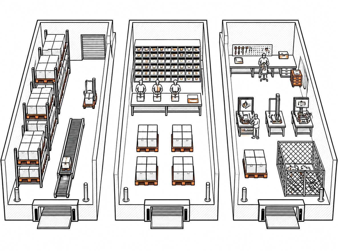
Editorial illustration of three warehouse floorplans side by side in cutaway: the first with a short belt and tall racking, the second with a dense sorting grid and a grading bench, the third with a refurbishment bench, testing rigs and a marked disposal cage, matching pallets and cartons in all three, flat hand-inked linework with light hatching.
The three roles differ in what they accept, what they judge, and where goods land, not in floor area

A specialized processing node exists to change the outcome rather than just move the unit. Refurbishment lines, functional testing, teardown for parts, and compliant destruction all live here. It can turn an unsellable return into a sellable one, which is worth real money on the right SKU, and it can retire an item safely when nothing else can. Its weakness is unit cost. Bench time and parts are expensive per piece, so it only makes sense above a value floor, and it is almost never the cheapest place to park a returned phone case.

The practical step is to build a capability table before you build a routing table. For each candidate node, record which categories it may accept, its grading depth, whether it can refurbish or only grade, its disposal or destruction permits, and its typical receiving queue in your busiest month. Routing decisions get much faster once that table exists, and merchant conversations get much shorter when you can say in one line why a unit went where it went.

Branch by reason first: no-fault returns vs. quality and damage

The return reason is a stronger predictor of the right node than the buyer's ZIP code. Two identical SKUs coming back for two different reasons should usually go to two different places, and forcing them down one path to simplify operations is how 3PLs end up with a grading backlog and disputed invoices.

A no-fault return is a change of mind, an ordered-by-mistake, a duplicate. The buyer is not alleging a defect, so there is usually nothing to adjudicate. Default sellable probability is high, the acceptance standard is wide, and the fastest path back to sellable inventory wins. That points at a direct-to-fulfillment warehouse whenever the goods are complete and the packaging is intact.

A quality or damage return is a different job. Someone has to open it, photograph it, and record what they found, because the finding decides who pays: a carrier claim, a supplier claim, or your own margin. That work needs an evidence bench and a written report, and it needs a node that can decide between refurbish, resell as-is, part out, and destroy. This is where centralized hubs and specialized nodes earn their place. It is also where the clock is different: for damage, the number that matters is days to a completed finding, because claim windows close while units sit in a queue. FedEx asks for a damage claim within 21 calendar days of delivery (FedEx claim window), and UPS within 60 days of the scheduled delivery date (UPS claim process). Neither window cares how long your grading queue is.

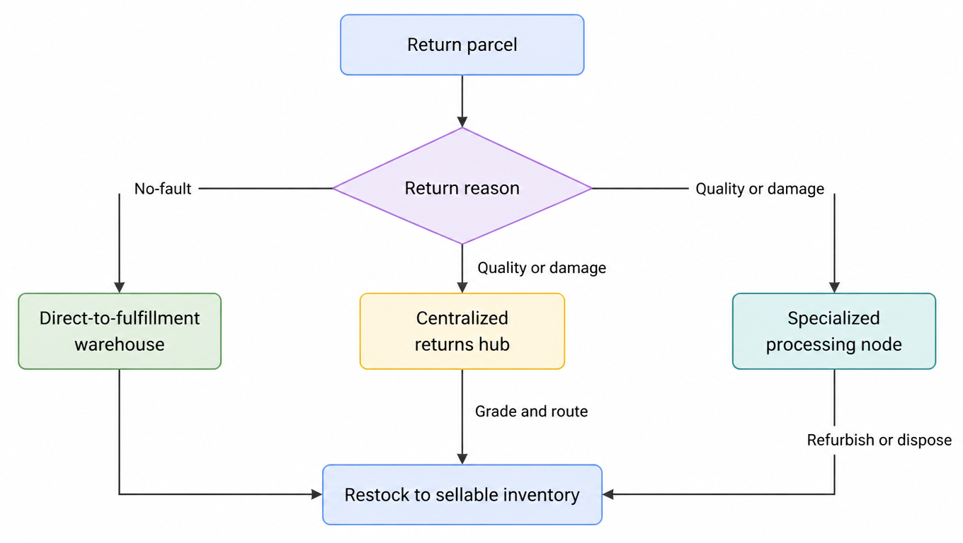
Flowchart: the return parcel branches first by reason, no-fault goes to a direct-to-fulfillment warehouse while quality or damage goes to a centralized returns hub or a specialized processing node, and all three lines converge on restocking to sellable inventory
Branch by reason first: the two lines have opposite default directions

Mixed shipments need a rule written down in advance. When one box holds three good units and one damaged one, the default of treating the whole box by its worst item silently writes off value, and the default of judging item by item without a cap destroys your receiving productivity. Pick a threshold, for example split the shipment when the damaged share exceeds a set fraction of units or of value, and put it in the service agreement.

The three cost lines: reverse freight, processing fee, transfer cost

The scorecard needs three cost lines side by side. Most routing mistakes come from comparing only the first one.

Return shipping is the buyer's ZIP to the candidate node, and the first question is who pays. If the merchant absorbs it, it lands on the merchant's line. If the buyer pays a flat rate, the difference between nodes lands on the buyer's, which changes the routing math but not the routing logic. Watch for a hidden lock-in: a pre-printed return label the merchant put in the box at ship time has already chosen the destination, so routing freedom only exists when the label is bound after the reason is known, either by the buyer through a portal or by the returns process itself. If your merchant clients are still shipping pre-printed labels, that is the first thing to fix, because it costs nothing and removes the entire decision from the return leg.

Processing fee is where a per-action schedule beats a single blended rate. Receiving and registration, grading, restocking, refurbishment, and disposal are different amounts of work with different labor and inputs, and quoting them separately lets a genuinely cheap path, like a complete return that skips deep inspection and goes straight to the shelf, show up as cheap. It also makes disputes shorter, because a merchant can see which action they are paying for.

Transfer cost is the line that gets forgotten, and it is the one that most often reverses the answer. A centralized hub may process a unit for less than a fulfillment warehouse, then spend the difference moving it to where it can actually be sold. Include the second leg explicitly, with its pooling or consolidation assumptions, and state in the agreement who carries it. Add the tail costs in the same table rather than in a footnote: long-dwell storage after a set number of days, re-labelling, a second open-and-inspect pass, and the time cost of a dock queue in peak season. Every one of these has a number, and the schedule is only credible if all of them are on it.

Restock time: days to sellable as a cost input

Time is not a soft metric. It enters the calculation as days, because days multiply the value of the goods. The relevant clock is not delivery time, it is days to sellable, and it has five segments: transit to the node, receiving and registration, the quality check queue, the disposition decision, and the restock itself.

Break the clock that way and the answer is usually humbling. On most returns the delay is not in transit. It is in the queue in front of the bench and in a disposition decision that nobody owns, which is why two nodes with the same carrier lane can differ by a week. This is also where a centralized hub's advantage can invert. Its grading consistency is real, but a peak-season backup at the receiving dock can add days to every unit in the building, and a nearby fulfillment warehouse with a short belt suddenly beats it on total score.

Measure the metric with the right denominator. Use returns initiated, not returns completed. If the denominator counts only units that finished the process, the ones that stalled, got lost, or were abandoned by the buyer disappear from the average and the number looks better than the operation is. Split it by node and by reason as well, because a single blended average hides the long tail that damage returns create. Agree on a baseline with each merchant, first-restock time, second-transfer rate, sellable rate, and report monthly against it. The report is what turns a routing rule into a managed service.

Expected recovery value and the combined route score

Recovery value is the return of the unit to something you can sell, and it should be computed before the comparisons, not after. Start from the value you can realistically realize, at the grade you expect, not the sticker price. A discounted resale price, a refurbished price, or a wholesale price for a graded lot are all valid inputs. List price is not, because it will make every route look profitable.

Two discipline rules keep the table honest. First, keep the incremental cash comparison of a disposition separate from full order-profit accounting. A return route can be cash positive and still be a loss on the original order, and mixing the two lets a real cost hide behind a refund that was going to be paid anyway. Second, keep the definitions consistent across refund, return shipping, and recoverable goods value, or you will deduct the same cost twice. If the return label is already charged as a cost line, it does not get subtracted a second time from the goods value.

The combined score then follows one line of arithmetic: route score = expected recovery value − return shipping − processing fee − transfer cost − (days to sellable × daily decay).

Daily decay is the term that translates slowness into money. It is the value a unit loses per day of delay, and it varies by category: seasonal goods fall off a cliff at the season boundary, electronics lose value as the next model ships, fast fashion ages by the week, and a plain steel bracket barely moves. Decay is also the term that makes a one-week difference between two nodes quantifiable instead of rhetorical.

When you do not have a reliable sell-through probability, do not reach for an industry average. Run scenarios, an optimistic, a base, and a pessimistic case, and report which routes hold up across all three. The decision rule after that is simple: a node must clear gate zero, then the highest score wins, and when two routes are within noise of each other, prefer the one with the steadier sellable probability and the shorter queue. And when a route fails on suitability, traceability, or compliance, it stops there. Do not average that failure away with a cheap rate.

Worked example: one SKU, two reasons, three node roles

Take a mid-value consumer electronics SKU with a rechargeable battery, about $64 of realizable value in good condition, with a daily decay of $0.26 per unit. Three candidate nodes: A, a direct-to-fulfillment warehouse near the buyer on the East Coast; B, a centralized returns hub in the Midwest; C, a specialized refurbishment node on the West Coast. Processing quotes follow a per-action schedule, and the buyer absorbs return shipping under the merchant's flat-rate policy, so the label is generated when the return is approved.

Line one, a no-fault return, complete and in original packaging. Grading is light, so sellable probability sits at 0.95 for all three.

Node Return shipping Processing Transfer Days to sellable Route score
A direct-to-fulfillment$7.80$2.70$0.006$48.74
B centralized hub$9.20$3.60$1.9011$43.24
C specialized (refurb)$12.40$4.20$2.6014$37.96

A wins, but notice how little of the win comes from the return leg. A is $4.60 cheaper than C on shipping and still beats it by nearly eleven dollars overall, because the hub and the refurb node each add a transfer and a queue that the direct route never pays for.

Line two, the same SKU arriving with a cracked housing. Node A is out at gate zero. It has no evidence bench and no functional test rig, so it cannot produce the finding that a carrier claim needs, and a cheap rate does not make it a candidate. B and C compete on their ability to turn the unit into something sellable: the hub puts a 0.55 chance on moving it as-is at $34, while the refurb node puts a 0.88 chance on a $64 refurbished unit after replacing the housing.

Node Return shipping Processing Transfer Days to sellable Route score
B centralized hub$9.20$6.10$0.009$1.06
C specialized (refurb)$12.40$13.80$2.6021$22.06

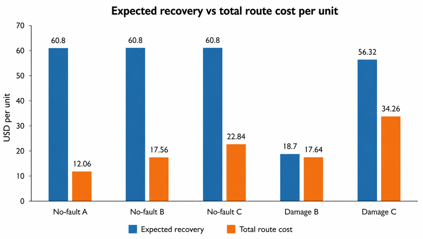
C wins by twenty-one dollars despite being the most expensive node on every single cost line, because a refurbished unit recovers $56 instead of the $34 that the hub can get for it as-is. This is the flip that reverse routing has and outbound routing does not: the cheapest leg loses.

Bar chart: expected recovery against total route cost per unit across five routes. The three no-fault routes each expect 60.8 dollars of recovery with total costs of 12.06, 17.56, and 22.84; damaged B is 18.7 against 17.64, and damaged C is 56.32 against 34.26
Expected recovery against total route cost under both reasons, hypothetical parameters rather than benchmarks

The sensitivity check is what you present to the merchant. Push the route in one case where A's peak-season queue stretches days to sellable from six to fifteen and it still wins, so that route is robust. Push it further, to a scenario where rushed grading drops A's sellable probability to 0.82, and B overtakes it, which tells you the decision is sensitive to grading quality, not to freight rates. Of the two dials in the model, sellable probability and daily decay, the probability estimate is almost always the shakier one, and it is the one worth investing in measuring.

What you hand over: a routing scorecard and a quote sheet

The internal deliverable is a routing scorecard. Rows are SKU and return reason, columns are candidate nodes, and each cell carries the four lines, the days to sellable, and a gate result with a reason if the node was excluded. Sellable probability and daily decay sit at the top as adjustable parameters so your team computes route scores from your own data instead of borrowing a benchmark that does not describe your network.

SKU × return reason Candidate node Gate result Return shipping Processing Transfer Days to sellable Expected recovery Route score
(fill in)————————
(fill in)————————
(fill in)————————

The external deliverable is a quote sheet that can go into a contract as an appendix. Build it on the per-action skeleton: receiving and registration, grading, restocking, refurbishment, disposal, each with its own price and its own definition of what is included. Then add the exception and dwell schedule, surcharges for oversize, battery-containing, liquid, unlabelled, and incomplete units, and long-dwell storage from a stated day. Write the billing basis in the same document: per return initiated, inclusive or exclusive of transfer, and when the dwell clock starts. Ambiguity in those three sentences causes more merchant disputes than any rate does.

Close the loop with a monthly report: first-restock time, second-transfer rate, sellable rate, and total cost per return initiated, split by node and by reason. A routing rule that is written down, measured, and invoiced with the same vocabulary stops being a negotiation and starts being a service. That is the difference between a merchant who calls you about every return and one who renews.

To actually run the scorecard, what is usually missing is data rather than a formula. For the RMA-to-unit match and the portal-to-WMS loop, see the reverse-logistics data model; for turning grading standards into repeatable actions, see returns shipping strategy for DTC brands and 3PLs; and for the outbound leg when a returned unit is simply reshipped to the next buyer, see the multi-warehouse order routing framework. The 3PL quote structure itself is covered in 3PL parcel pricing models. Before you commit, size the reverse leg with the shipping rate calculator and check where execution cost lands against pricing; the wider picture is in ecommerce shipping solutions, whether to systemize is covered in evaluating returns software, and the returns that should never come back at all are covered in the box-free vs. QR-code vs. mail-in comparison.

Make the reverse leg a number you can compute too

EasyShippingX is a channel-neutral shipping layer: it compares US carrier options in one place and executes them through the Portal, Excel, or the API. A returned parcel and the next outbound order run on the same quoting logic, so you can price both directions with the same inputs before deciding which node should receive each tier of return.